A smooth Introduction to Portfolio Management
Introduction to Portfolio Management
In this short blog I am going to introduce the basics of portfolio
theory. It is an introduction to a set of blogs dedicated to
portfolio choices that focus on long holding
periods. In particular, these periods are between 10 and 30
years. Several studies revealed that frequently switching between funds
leads investors to withdraw from and invest into the market at wrong
times. This implies that market-timing does not work for the average
investor. Dalbar for instance, publishes continuous reports on “Quantitative
Analysis of Investor Behavior” that support the idea that short-term
investing might lead to make the exact wrong decision. The definitions
below will help to build methodologies for a systematic approach to
investing. I will try to keep everything as short as possible.
So
lets start with the risk-return tradeoff, which is the
principle that expected return rises with an increase in risk. Thus, an
investor can expect higher profits only if the investor is willing to
accept the possibility of higher losses. Markowitz (1991) shows how to
maximize expected return for a given level of variance. He assumes that
investors prefer asset A over B with same expected return, whenever
asset A has a smaller variance than asset B.
Definitions
In order to get a logical understanding of the topic and developing it further, we need to make some definitions that will be referred to across posts. First and foremost, the portfolio return is defined as: \[ r_p = \sum_{i=1}^n w_i r_i = w'r \] with weights summing up to 1: \[ \sum_{i=1}^n w_i = w' 1\]
The expected return of a portfolio is \[\mu_p = \mathop {\mathbb E}[r_p] =
\sum_{i=1}^n w_i \mathop {\mathbb E}[r_i] = w' \mathop {\mathbb
E}[r]\] and the corresponding variance of the portfolio
return is: \[ \sigma_p^2 =
\sum_{i=1}^n w_i^2 \sigma_i^2 + \sum_{i=1}^n\sum_{i\neq j} w_i
w_j Cov[r_i, r_j] = w'\Sigma w\]
Diversification
The last equation reveals that portfolio risk consists of two
components. The first part is called idiosyncratic
risk and is almost fully diversifiable. In general,
diversification is a technique that reduces risk by allocating
investments among various financial instruments, industries, and other
categories. It aims to maximize return by investing in different areas
or assets that are expected to move in different directions given a
specific shock. As a result, idiosyncratic risks are
risks specific to a company, industry, market, economy, or country are
reduced, if not eliminated. The concept of diversification can also be
shown by a mathematical proof, which is derived in only one line.
Proof:
For this purpose we assume a zero covariance, meaning that the
correlation between assets is zero. If we use an equally weighted
portfolio, such that \(w_i = 1/n\),
then the portfolio’s variance will converge to zero as n goes to
infinity. Most ETFs on indices however are value-weighted and
automatically introduce exposure to a value risk premium, which might
not be intended by the investor. In particular, the proof below would
also hold for a value-weighted portfolios as the weights would be a
function of individual market capitalization and \(n\), such that \((w_i = MC_i/(\overline{MC}\cdot n)\). Thus
the portfolio variance converges slower to 0 as \(n\) grows linearly instead of
exponentially.
\[\lim_{n \to \infty} \sigma_p^2 = \lim_{n
\rightarrow \infty} \sum_{i=1}^n \frac{ \sigma_i^2} {n^2} +
\sum_{i=1}^n\sum_{i\neq j} \frac{ 0} {n^2}= 0\] We can see that
it is desirable to benefit from the diversification
effect which reduces portfolio risk.
Geometric Proof:
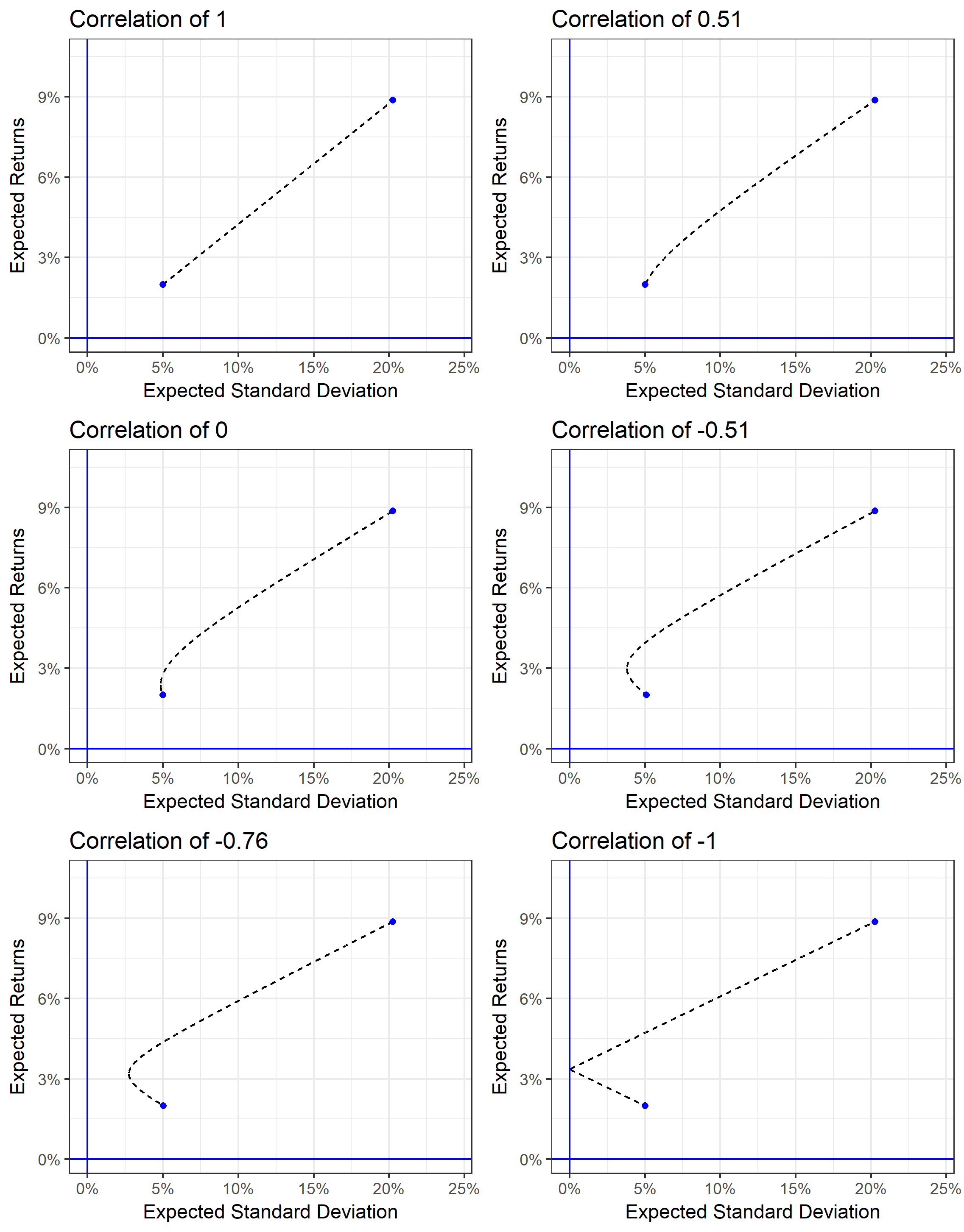
The second part of the portfolio variance is the weighted covariance. This part can also be represented by entries of the correlation matrix multiplied by the standard deviation. Hence, any correlation contributes positively or negatively to the overall portfolio risk. For illustration purposes consider the plot below: It shows two assets with various return correlations. The blue dots indicate a full investment in either one of the two assets. Further, the dashed line indicates all possible portfolios constructed by these two assets. Only if the correlation is perfectly negative, the portfolio risk will be zero.
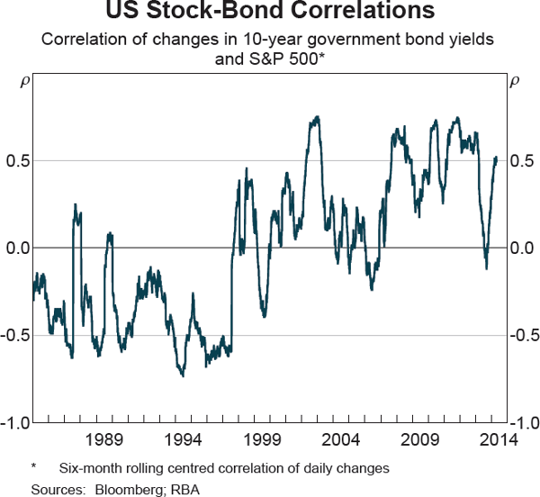
Unfortunately, zero correlations across assets are unobservable (see
also US Stock-Bond plot) and thus, the second part of the portfolio
variance is unequal to zero. In general, systematic
risks are variations in inflation rates and exchange rates,
political and economic instability, war, and interest rate changes,
which is undiversifiable. Nonetheless, the latter risk
component is supposed to be priced in financial markets and is the
compensation for bearing systematic risks. This compensation is known as
the risk premium or discount rate. These discount rates
are time varying as a result of time variation in the underlying
portfolio return correlations. Idiosyncratic risk on the other hand, is
not compensated as it is diversifiable.
Obviously, if the
last part is negative, the entire variation is smaller, which is the
main idea of the 60/40 asset allocation rule that invests in stocks and
bonds. The idea thereby is that the two asset classes generally move in
opposite directions and are thus negatively correlated. Unfortunately,
since 1999, the negative relationship has turned positive for long-term
holdings as plotted above.
Fortunately, a very large set of different approaches exists that try
to implement low correlations with the market and simultaneously take
advantage of the diversification effect. Some of these methodologies are
discussed in later sections. These examples try to optimize the
trade-off between risk and return, but also wrt higher moments. Some of
these methods also consider reduced transaction costs by decreasing the
turnover or the number of assets n as there exists an obvious trade-off
between high diversification, implying a large number of assets \(n\), and fees.
Before we jump to MV
estimation we should mention the behavior of discount rates.
Surprisingly, it turned out that expected stock returns are
time-varying in contrast to the view of the 1970s. As a
consequence, discount rate variation over time and across assets has
replaced informational efficiency as the central
organizing question of asset pricing. Several arguments try to explain
the time variation:
- Campbell and Cochrane (1999): time-varying risk aversion
- Bansal and Yaron (2004): time-varying diffusive risk
- Wachter (2013): time-varying disaster risk
Although, we are not completely confident what causes time-variation, we should bear in mind that expectations estimated via the short to medium run might be better approximations for expected returns than long run measures.