Geometric Beta: Projection, Orthogonality, and Market Geometry
Overview
Traditional beta collapses asset–market relationships into a single scalar. This obscures how an asset differs from the market.
Geometric beta decomposes asset behavior into:
- Scalar alignment with the market (crowd risk)
- Orthogonal divergence from the market (structural or diversifying risk)
This document formalizes the mathematics and provides geometric intuition.
1. Vector Space Representation of Returns
Let returns over a rolling window of \(N\) days be represented as vectors:
\[ \mathbf{m} = (m_1, m_2, \dots, m_N) \in \mathbb{R}^N \]
\[ \mathbf{a} = (a_1, a_2, \dots, a_N) \in \mathbb{R}^N \]
Each coordinate corresponds to time, not a factor. This is geometry in trajectory space.
2. Scalar Beta (Projection onto the Market)
Definition
The scalar beta is the projection of the asset vector onto the market vector:
\[ \beta_{\text{scalar}} = \frac{\mathbf{a} \cdot \mathbf{m}}{\mathbf{m} \cdot \mathbf{m}} \]
Interpretation
- Measures how much of the asset’s movement is explained by the market
- Equivalent to CAPM beta when returns are demeaned
- Represents crowd participation
Geometric Meaning
Scalar beta is the shadow of the asset vector on the market axis.
If: \[ \mathbf{a} = k \mathbf{m} \]
then: - \(\beta_{\text{scalar}} = k\) - Asset is a pure market clone
3. Bivector Beta (Orthogonal Rejection)
Rejection Vector
Remove the market-aligned component:
\[ \mathbf{r} = \mathbf{a} - \beta_{\text{scalar}} \mathbf{m} \]
Bivector Beta
Normalize the magnitude of the rejection:
\[ \beta_{\text{bivector}} = \frac{\|\mathbf{r}\|}{\|\mathbf{m}\|} \]
Interpretation
- Measures movement independent of the market
- Captures structural, idiosyncratic, or regime-specific behavior
- Represents diversification geometry, not volatility
Key Property
If: \[ \mathbf{a} \cdot \mathbf{m} = 0 \]
then: - \(\beta_{\text{scalar}} = 0\) - Asset is purely orthogonal to the market
4. Exterior Algebra Interpretation
Wedge Product
The exterior (wedge) product:
\[ \mathbf{a} \wedge \mathbf{m} \]
represents the oriented area spanned by the two vectors.
Magnitude:
\[ \|\mathbf{a} \wedge \mathbf{m}\| = \sqrt{(\mathbf{a}\cdot\mathbf{a})(\mathbf{m}\cdot\mathbf{m}) - (\mathbf{a}\cdot\mathbf{m})^2} \]
3.1 Two-Dimensional Geometric Illustration
To build intuition, we visualize the asset–market relationship in two dimensions. The horizontal axis represents the market direction and the vertical axis represents the orthogonal (non-market) direction.
This is a geometric abstraction — the real vectors live in high-dimensional return space, but the relationships are identical.
# Define simple 2D vectors
market <- c(1, 0)
asset <- c(0.8, 0.6)

# Scalar beta (projection)
beta_scalar <- sum(asset * market) / sum(market * market)
projection <- beta_scalar * market

# Rejection (bivector component)
rejection <- asset - projection

# Plot setup
plot(
    c(0, 1.2),
    c(0, 1.0),
    type = "n",
    xlab = "Market Direction",
    ylab = "Orthogonal Direction",
    main = "Geometric Beta Decomposition",
    asp = 1
)

# Market vector
arrows(0, 0, market[1], market[2], lwd = 2, col = "black")
text(1, 0.05, "Market", pos = 4)

# Asset vector
arrows(0, 0, asset[1], asset[2], lwd = 2, col = "darkgreen")
text(asset[1], asset[2], "Asset", pos = 4)

# Projection (scalar beta)
arrows(0, 0, projection[1], projection[2], lwd = 2, col = "blue")
text(projection[1] * .6, 0.025, "Scalar Beta", col = "blue", pos = 3)

# Rejection (bivector beta)
arrows(
    projection[1],
    projection[2],
    asset[1],
    asset[2],
    lwd = 2,
    col = "red"
)
text(
    projection[1] + rejection[1] / 2,
    projection[2] + rejection[2] / 2,
    "Bivector Beta",
    col = "red",
    pos = 4
)

# Origin
points(0, 0, pch = 16)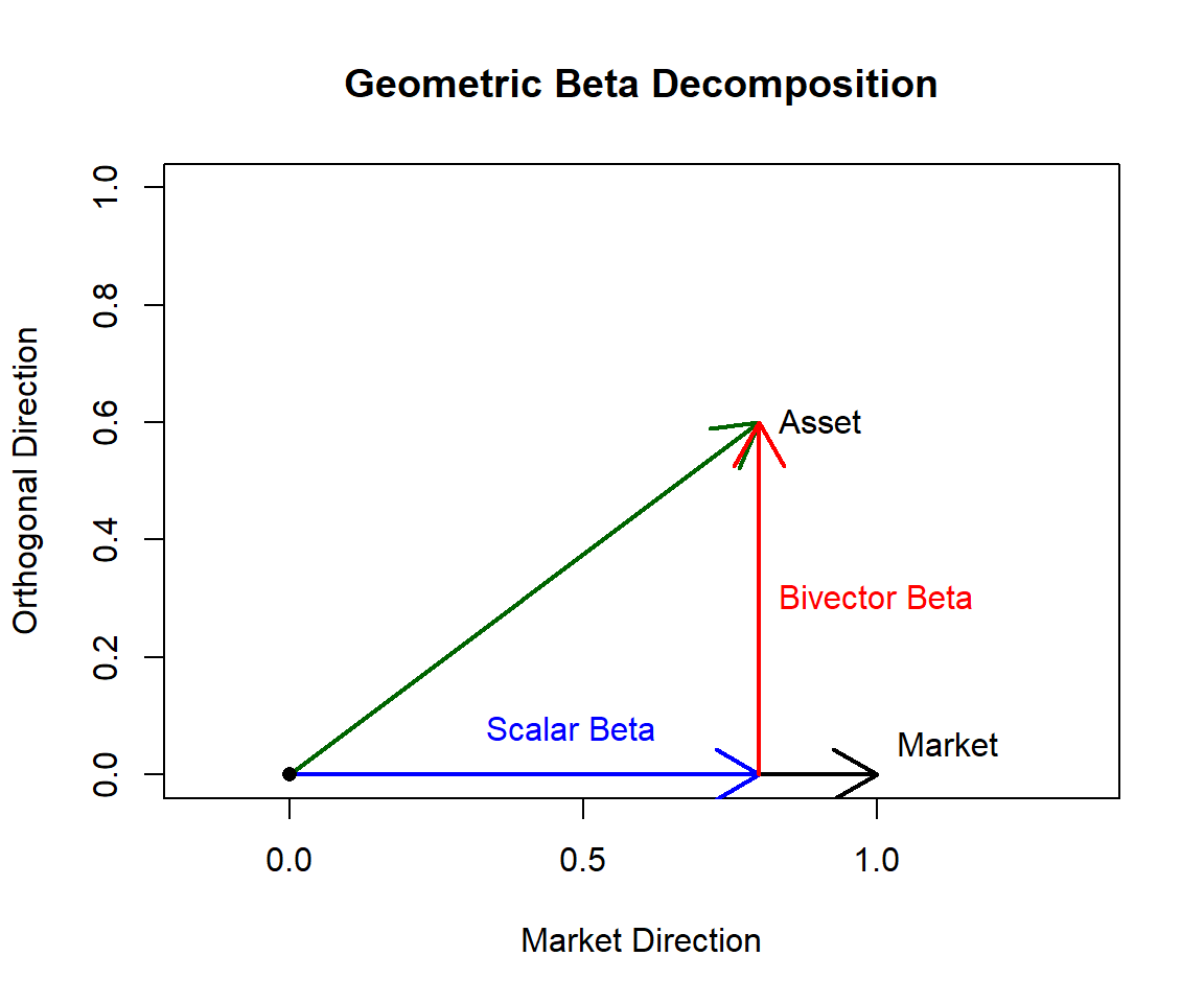
Equivalence
The rejection-based bivector beta satisfies:
\[ \|\mathbf{a} \wedge \mathbf{m}\| = \|\mathbf{m}\|^2 \cdot \beta_{\text{bivector}} \]
Thus:
- Scalar beta → grade-0 (inner product)
- Bivector beta → grade-2 (area element)
5. Relationship to PCA
| PCA | Geometric Beta |
|---|---|
| Rotates coordinate system | Fixes market direction |
| Variance-based | Orientation-based |
| Symmetric | Asymmetric (market-anchored) |
| Unstable in crises | Stable under regime stress |
PCA asks: > “What directions explain variance?”
Geometric beta asks: > “How much does this asset escape the market direction?”
6. Crisis Dynamics and Early Warning
Before correlation collapses:
- Market volatility rises
- Some assets rotate away from the market
- Bivector beta spikes
- Correlations later snap to one
Correlation reacts after geometry collapses. Bivector beta reacts during geometric divergence.
7. Intuition Summary
- Scalar beta: How much you move with the crowd
- Bivector beta: How different your path is
- Volatility: How fast you move
- Correlation: Average angle
- Geometry: Dimensional structure
Geometric beta decomposes asset risk into market-aligned motion and orthogonal structural motion, enabling regime-aware diversification based on geometry rather than correlation.
8. Application - Multiasset Portfolio Construction
Modern portfolio theory failed during several episodes of significant drawdowns as diversifiaction collapsed and all assets within the portfolio went sour. The most recent event was the drawdown in 2022, the “Everything Crash”. The reason is that risk metrics—correlation and traditional beta’s are geometrically incomplete. When inflation surged and interest rates reset, both equities and bonds declined simultaneously, revealing that conventional diversification relied on flat statistics that collapse under regime stress.
This framework replaces correlation-based thinking with Geometric Investing, which treats markets as high-dimensional geometric objects rather than collections of pairwise relationships. Returns over time are represented as vectors, and risk is analyzed through orientation, area, and volume instead of variance alone.
The approach is built on three geometric sensors:
- Geometric Beta Decomposes asset risk into:
- Scalar Beta: market-aligned (crowd) risk
- Bivector Beta: orthogonal, structurally independent risk This distinguishes assets that merely track the market from those that occupy genuinely independent dimensions of return space.
- Wedge Volume (Regime Detection) Measures the
hyper-volume spanned by sector return vectors using the Gram
determinant.
- High volume indicates a healthy, diversified market
- Low volume signals dimensional collapse and correlation convergence
- Orientation (Trend Validation) Uses the wedge product of time and price to determine the directional “spin” of an asset’s trajectory. Only assets with positive orientation (upward spin) are eligible for allocation, regardless of their geometric uniqueness.
Combined, these sensors form the Geometric Beta Portfolio, which dynamically rotates between equities, defensive assets, and cash based purely on geometric structure—without relying on traditional technical indicators.
Empirical results since 2010 show that the strategy: - Fully participates in bull markets - Rapidly de-risks during structural collapses (e.g., 2020) - Avoids major drawdowns during correlation crises (e.g., 2022)
The broader implication is that geometry provides a scalable language for risk. Just as flat statistics fail in finance, naive vector operations fail in other high-dimensional systems such as machine learning. Measuring and managing shape rather than averages offers a more robust foundation for complex decision-making.
Implementation notes (revised backtest)
The backtest below contains two corrections that apply to both variants:
- Bug fix — execution timing: decisions are made on the monthly close but earn returns only from the next day onward. The original booked the decision day’s return although the signals already used that day’s close (~1.1% p.a. look-ahead bias).
- Bug fix — dead code: the unused NNLS “dynamic gravity” block, the scalar-beta frame, and an unused rolling window were removed.
The two strategy variants
Both variants share the identical geometric core — wedge-volume regime detection (PANIC below the rolling 15th percentile, DEFENSE below the 40th), the 200-day orientation filter, and monthly rebalancing. They differ only in which defensive asset they buy and how much market exposure they take in OFFENSE:
Bivector.Unlevered — the pure geometric
specification.
- Defensive asset (TLT vs GLD): the one with the largest bivector beta \(\|\mathbf{r}\|/\|\mathbf{m}\|\), i.e. the asset currently most orthogonal to the market in magnitude terms.
- OFFENSE: 100% SPY, no leverage.
Momentum.Levered — the return-oriented
specification.
- Defensive asset: the one with the higher 12-1 momentum (12-month return excluding the most recent month). Geometry still decides when to defend; momentum decides what to hold.
- OFFENSE: 1.25× SPY, the excess 25% financed at the cash (SHV) rate.
Differences, advantages, and disadvantages
Bivector.Unlevered |
Momentum.Levered |
|
|---|---|---|
| Defensive pick | Largest orthogonal magnitude | Strongest trend |
| Market exposure in OFFENSE | 1.00× | 1.25× |
| CAGR / Sharpe / MaxDD (2010–2023) | 9.1% / 0.77 / 18.7% | 11.4% / 0.82 / 21.9% |
Bivector.Unlevered — advantages: conceptually
pure (every decision is geometric), no leverage, hence no financing
cost, no margin requirements, and the lowest volatility (≈12%) and
drawdown of the three series. Disadvantages: the bivector magnitude
scales with the asset’s own volatility, so it
systematically favors the most volatile diversifier rather than
the most rewarding one — the orientation filter only slowly vetoes a
deteriorating pick. Running at ~12% volatility against a ~17% benchmark,
it cannot keep up with the market in long bull phases despite its higher
Sharpe ratio.
Momentum.Levered — advantages: the defensive
sleeve holds the asset that is actually being paid (≈ +0.6% p.a. from
the pick alone), and the modest OFFENSE leverage converts the strategy’s
Sharpe advantage into absolute return — it beats the buy-and-hold
benchmark while still cutting the maximum drawdown roughly in half.
Crisis protection is untouched because leverage applies only in OFFENSE.
Disadvantages: it mixes a non-geometric ingredient (momentum) into the
framework; it requires a leverage implementation (futures or margin)
with financing-cost risk when short rates rise; and the 1.25× exposure
amplifies whipsaw losses around OFFENSE↔︎BEAR transitions, giving
slightly higher volatility and drawdown.
In short: Bivector.Unlevered is the cleaner
risk-management product, Momentum.Levered the
better total-return product at a still markedly lower risk than
the benchmark.
library(quantmod)
library(zoo)
library(PerformanceAnalytics)

########################################.
#######  1. GEOMETRIC OPERATORS  #######
########################################.

calculate_wedge_volume <- function(returns, window = 60) {
    vols <- numeric()
    dates <- index(returns)[(window + 1):nrow(returns)]
    r_val <- coredata(returns)

    for (i in seq(window + 1, nrow(r_val))) {
        win <- r_val[(i - window):(i - 1), , drop = FALSE]

        norms <- apply(win, 2, function(x) sqrt(sum(x^2)))
        norms[norms == 0] <- 1e-8
        norm_win <- sweep(win, 2, norms, "/")

        gram <- t(norm_win) %*% norm_win
        vols <- c(vols, sqrt(abs(det(gram))))
    }

    return(xts(vols, order.by = dates))
}


calculate_geometric_beta <- function(asset_returns, market_returns, window = 60) {
    dates <- index(asset_returns)[(window + 1):nrow(asset_returns)]
    scalar <- numeric()
    bivector <- numeric()

    a <- coredata(asset_returns)
    m <- coredata(market_returns)

    for (i in seq(window + 1, length(a))) {
        vec_a <- a[(i - window):(i - 1)]
        vec_m <- m[(i - window):(i - 1)]

        m_sq <- sum(vec_m^2)
        if (m_sq == 0) {
            m_sq <- 1e-8
        }

        sc <- sum(vec_a * vec_m) / m_sq
        rej <- vec_a - sc * vec_m
        bi <- sqrt(sum(rej^2)) / sqrt(m_sq)

        scalar <- c(scalar, sc)
        bivector <- c(bivector, bi)
    }

    return(list(
        scalar = xts(scalar, order.by = dates),
        bivector = xts(bivector, order.by = dates)
    ))
}


calculate_bivector_orientation <- function(prices, window = 200) {
    return(diff(prices, lag = window) > 0)
}


########################################.
#######  2. STRATEGY EXECUTION  ########
########################################.

runGMM <- function(start_date = "2010-01-01", end_date = "2024-01-01") {
    sectors <- c("XLK", "XLF", "XLV", "XLE", "XLI", "XLY", "XLP", "XLB", "XLU")
    assets <- c("SPY", "TLT", "GLD")
    cash <- "SHV"
    tickers <- c(sectors, assets, cash)

    getSymbols(tickers, from = start_date, to = end_date, auto.assign = TRUE)

    prices <- do.call(merge, lapply(tickers, function(t) Ad(get(t))))
    colnames(prices) <- tickers
    returns <- na.omit(diff(log(prices)))

    spy <- returns$SPY
    sec_ret <- returns[, sectors]

    wedge_vol <- calculate_wedge_volume(sec_ret, 60)
    defense_thresh <- rollapply(wedge_vol, 252, quantile, probs = 0.40, fill = NA)
    panic_thresh <- rollapply(wedge_vol, 252, quantile, probs = 0.15, fill = NA)

    # Build bivector_df via list then merge (empty-xts column assignment fails)
    gb_results <- lapply(setNames(assets, assets), function(a) {
        calculate_geometric_beta(returns[, a], spy, 60)
    })
    bivector_df <- do.call(merge, lapply(gb_results, `[[`, "bivector"))
    colnames(bivector_df) <- assets

    orientations <- do.call(
        merge,
        lapply(setNames(tickers, tickers), function(t) {
            calculate_bivector_orientation(prices[, t], 200)
        })
    )
    colnames(orientations) <- tickers

    # 12-1 momentum, used by the improved variant's defensive pick
    mom12 <- do.call(
        merge,
        lapply(setNames(tickers, tickers), function(t) {
            diff(log(prices[, t]), lag = 252) - diff(log(prices[, t]), lag = 21)
        })
    )
    colnames(mom12) <- tickers

    # Intersect indices without stripping Date class
    idx <- index(wedge_vol)[
        index(wedge_vol) %in% index(bivector_df) & index(wedge_vol) %in% index(orientations)
    ]
    # Last trading day of each month
    monthly <- idx[!duplicated(format(idx, "%Y-%m"), fromLast = TRUE)]

    run_variant <- function(pick = c("bivector", "momentum"), offense_lev = 1) {
        pick <- match.arg(pick)
        holdings <- c(SPY = 1)
        history <- data.frame(date = as.Date(character()), mode = character(), stringsAsFactors = FALSE)
        port_ret <- numeric(length(idx))

        # seq_along preserves Date/POSIXct class when subsetting idx[i]
        for (i in seq_along(idx)) {
            d <- idx[i]

            # Book the day's return BEFORE the (monthly) decision: the signals use
            # the close of d, so new weights may only earn from d+1 (no look-ahead)
            port_ret[i] <- sum(holdings * as.numeric(returns[d, names(holdings)]))

            if (d %in% monthly) {
                vol <- as.numeric(wedge_vol[d])
                pth <- as.numeric(panic_thresh[d])
                dth <- as.numeric(defense_thresh[d])

                if (!is.na(vol) && !is.na(pth) && vol < pth) {
                    holdings <- setNames(1, cash)
                    mode <- "PANIC"
                } else if (!is.na(vol) && !is.na(dth) && vol < dth) {
                    cands <- c("TLT", "GLD")
                    orient_vals <- as.logical(orientations[d, cands])
                    valid <- cands[!is.na(orient_vals) & orient_vals]

                    if (length(valid) > 0) {
                        score <- switch(pick, bivector = as.numeric(bivector_df[d, valid]), momentum = as.numeric(mom12[d, valid]))
                        score[is.na(score)] <- -Inf
                        best <- valid[which.max(score)]
                        holdings <- setNames(1, best)
                        mode <- paste("DEFENSE", best)
                    } else {
                        holdings <- setNames(1, cash)
                        mode <- "DEFENSE FAILED"
                    }
                } else {
                    spy_up <- isTRUE(as.logical(orientations[d, "SPY"]))
                    if (spy_up) {
                        # offense_lev > 1 borrows at the cash (SHV) rate
                        holdings <- c(SPY = offense_lev, setNames(1 - offense_lev, cash))
                        holdings <- holdings[holdings != 0]
                        mode <- "OFFENSE"
                    } else {
                        holdings <- setNames(1, cash)
                        mode <- "BEAR"
                    }
                }
                history <- rbind(history, data.frame(date = as.Date(d), mode = mode, stringsAsFactors = FALSE))
            }
        }

        list(ret = xts(port_ret, order.by = idx), history = history)
    }

    bivector_unlevered <- run_variant("bivector", offense_lev = 1)
    momentum_levered <- run_variant("momentum", offense_lev = 1.25)

    strat <- merge(bivector_unlevered$ret, momentum_levered$ret)
    bench <- xts(as.numeric(spy[idx]), order.by = idx)
    colnames(strat) <- c("Bivector.Unlevered", "Momentum.Levered")
    colnames(bench) <- "Benchmark"

    list(
        strategy = strat,
        benchmark = bench,
        history_bivector = bivector_unlevered$history,
        history_momentum = momentum_levered$history
    )
}

########################################.
##########  3. VISUALIZATION  ##########
########################################.

plot_helper <- function(strat, bench, history) {
    charts.PerformanceSummary(
        merge(strat, bench),
        legend.loc = "topleft",
        main = "Pure Geometric Fortress"
    )
}

res <- runGMM()
plot_helper(res$strategy, res$benchmark, res$history_bivector)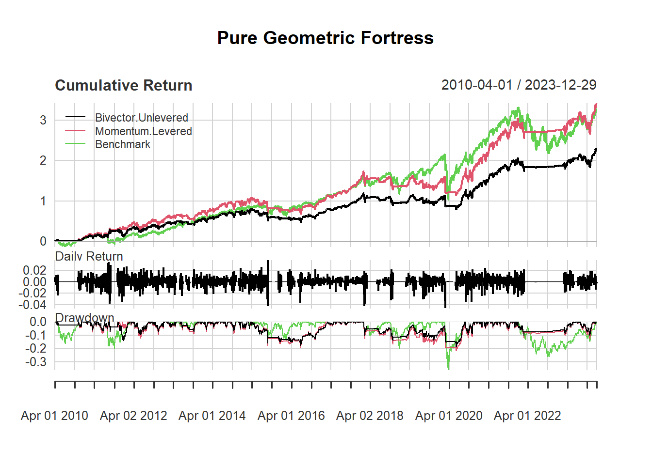
perf <- merge(res$strategy, res$benchmark)
rbind(
    CAGR = round(Return.annualized(perf) * 100, 2),
    Vol = round(StdDev.annualized(perf) * 100, 2),
    Sharpe = round(SharpeRatio.annualized(perf, Rf = 0), 2),
    MaxDD = round(maxDrawdown(perf) * 100, 2)
)
## Bivector.Unlevered Momentum.Levered Benchmark
## Annualized Return 9.07 11.39 11.14
## Annualized Standard Deviation 11.78 13.97 17.43
## Annualized Sharpe Ratio (Rf=0%) 0.77 0.82 0.64
## Worst Drawdown 18.70 21.86 35.75