Path-Dependent Volatility: Guyon & Lekeufack (2023)

Summary, In-Sample Regression, and Out-of-Sample Forecasting in R

Author

Gabriel Kaiser

Published

June 8, 2026

Model Summary

Overview

Guyon & Lekeufack (2023) — “Volatility Is (Mostly) Path-Dependent” — show that roughly 90% of S&P 500 implied volatility dynamics can be explained by the price path alone, without any news or macro inputs.

The model regresses current volatility on two path-derived features:

\[ \text{Vol}_t = \beta_0 + \beta_1 R_{1,t} + \beta_2 \sqrt{R_{2,t}} \]

where:

\[ R_{1,t} = \sum_{s=1}^{K} K_1(s)\, r_{t-s} \qquad \text{(trend / leverage)} \]

\[ R_{2,t} = \sum_{s=1}^{K} K_2(s)\, r_{t-s}^2 \qquad \text{(activity / clustering)} \]

\(\beta_1 < 0\) — drawdowns push volatility up (leverage effect)
\(\beta_2 > 0\) — elevated past squared returns raise current vol (clustering)

Kernel Choice

The paper evaluates two kernel families:

Kernel	Formula	Parameters
Exponential	\(K(\tau) = \lambda e^{-\lambda \tau}\)	\(\lambda > 0\) (decay rate)
Time-shifted power law (TSPL)	\(K(\tau) = Z^{-1}(\tau + \delta)^{-\alpha}\)	\(\alpha > 1\), \(\delta > 0\)

TSPL kernels produce heavier-tailed memory and better fit empirical volatility.

Roughness Claim

Rough volatility models posit a fractional Brownian motion with \(H \approx 0.1\). Guyon & Lekeufack show their model — with plain exponential kernels — produces a signal that looks equally rough, suggesting the roughness may be a spurious artifact of path-dependency, not a true fractional process.

Helper Functions

Code

# ----------------------------------------------------------------
# Exponential kernel: K(tau) = lambda * exp(-lambda * tau)
# ----------------------------------------------------------------
exp_kernel <- function(lambda, K) {
    tau <- seq_len(K)
    w <- lambda * exp(-lambda * tau)
    w / sum(w)
}

# ----------------------------------------------------------------
# Time-shifted power law: K(tau) = (tau + delta)^{-alpha}
# ----------------------------------------------------------------
tspl_kernel <- function(alpha, delta, K) {
    tau <- seq_len(K)
    w <- (tau + delta)^(-alpha)
    w / sum(w)
}

# ----------------------------------------------------------------
# Compute R1 and R2 using a given kernel function
# Uses stats::filter() for speed
# ----------------------------------------------------------------
compute_features <- function(r, kernel_fn, K = 252) {
    w <- kernel_fn(K)
    r2 <- r^2

    R1 <- as.numeric(stats::filter(r, w, sides = 1))
    R2 <- as.numeric(stats::filter(r2, w, sides = 1))

    data.frame(
        t = seq_along(r),
        R1 = R1,
        R2 = R2,
        Sigma = sqrt(pmax(R2, 0))
    )
}

# ----------------------------------------------------------------
# 21-day rolling realized volatility (annualized)
# ----------------------------------------------------------------
roll_vol <- function(r, window = 21, ann = 252) {
    n <- length(r)
    rv <- rep(NA_real_, n)
    for (i in (window + 1):n) {
        rv[i] <- sd(r[(i - window):(i - 1)]) * sqrt(ann)
    }
    rv
}

# ----------------------------------------------------------------
# Hurst exponent via R/S analysis (pracma)
# ----------------------------------------------------------------
compute_hurst <- function(x) {
    x <- x[!is.na(x)]
    h <- pracma::hurstexp(x, display = FALSE)
    list(Hs = h$Hs, Hrs = h$Hrs, He = h$He)
}

In-Sample Regression (Paper Application)

Synthetic Data

Code

set.seed(42)
T_sim <- 2500
dates <- seq.Date(as.Date("2015-01-05"), by = "day", length.out = T_sim)

# GARCH(1,1): omega=1e-6, alpha=0.08, beta=0.90
sigma2 <- numeric(T_sim)
r_sim <- numeric(T_sim)
sigma2 <- 1e-6 / (1 - 0.08 - 0.90)[1]
r_sim <- rnorm(1, 0, sqrt(sigma2))[1]

for (t in 2:T_sim) {
    sigma2[t] <- 1e-6 + 0.08 * r_sim[t - 1]^2 + 0.90 * sigma2[t - 1]
    r_sim[t] <- rnorm(1, 0, sqrt(sigma2[t]))
}

true_vol <- sqrt(sigma2) * sqrt(252)
realized_vol <- roll_vol(r_sim, window = 21)

cat(sprintf("T = %d | mean RV = %.4f | sd RV = %.4f\n", T_sim, mean(realized_vol, na.rm = TRUE), sd(realized_vol, na.rm = TRUE)))

T = 2500 | mean RV = 0.1031 | sd RV = 0.0385

Exponential Kernels

Code

BURN <- 30
K <- 252

lambda1 <- 0.05
lambda2 <- 0.20

feats_exp <- compute_features(
    r_sim,
    kernel_fn = function(K) exp_kernel(lambda1, K),
    K = K
)

df_exp <- data.frame(vol = realized_vol, R1 = feats_exp$R1, Sigma = feats_exp$Sigma, date = dates) |>
    slice(-(1:BURN)) |>
    na.omit()

fit_exp <- lm(vol ~ R1 + Sigma, data = df_exp)
df_exp$fitted <- fitted(fit_exp)

cat("=== Exponential Kernels ===\n")

=== Exponential Kernels ===

Code

print(summary(fit_exp)$coefficients)

               Estimate   Std. Error    t value     Pr(>|t|)
(Intercept) -0.00611243 0.0007755484  -7.881430 5.001715e-15
R1           1.95494932 0.2168962062   9.013294 4.170254e-19
Sigma       16.57597899 0.1114386515 148.745330 0.000000e+00

Code

cat(sprintf("\nR² = %.4f\n", summary(fit_exp)$r.squared))


R² = 0.9155

TSPL Kernels (Paper Specification)

Code

alpha1 <- 1.06
delta1 <- 0.020
alpha2 <- 1.60
delta2 <- 0.052

feats_tspl <- compute_features(
    r_sim,
    kernel_fn = function(K) tspl_kernel(alpha1, delta1, K),
    K = K
)
Sigma_tspl <- sqrt(pmax(
    as.numeric(stats::filter(r_sim^2, tspl_kernel(alpha2, delta2, K), sides = 1)),
    0
))

df_tspl <- data.frame(vol = realized_vol, R1 = feats_tspl$R1, Sigma = Sigma_tspl, date = dates) |>
    slice(-(1:BURN)) |>
    na.omit()

fit_tspl <- lm(vol ~ R1 + Sigma, data = df_tspl)
df_tspl$fitted <- fitted(fit_tspl)

cat("=== TSPL Kernels (paper VIX params) ===\n")

=== TSPL Kernels (paper VIX params) ===

Code

print(summary(fit_tspl)$coefficients)

              Estimate  Std. Error   t value      Pr(>|t|)
(Intercept) 0.04235184 0.001411687 30.000874 1.378608e-166
R1          1.28714061 0.349734713  3.680334  2.384140e-04
Sigma       9.60099610 0.202334649 47.451073  0.000000e+00

Code

cat(sprintf("\nR² = %.4f\n", summary(fit_tspl)$r.squared))


R² = 0.5095

Model Comparison Table

Code

betas = coef(fit_exp)
betasFit = coef(fit_tspl)
tibble::tibble(
    Kernel = c("Exponential", "TSPL (paper)"),
    beta0 = c(betas[1], betasFit[1]),
    beta1 = c(betas[2], betasFit[2]),
    beta2 = c(betas[3], betasFit[3]),
    R2 = c(summary(fit_exp)$r.squared, summary(fit_tspl)$r.squared)
) |>
    mutate(across(where(is.numeric), round, 5)) |>
    knitr::kable(caption = "In-sample regression summary")

In-sample regression summary
Kernel	beta0	beta1	beta2	R2
Exponential	-0.00611	1.95495	16.57598	0.91545
TSPL (paper)	0.04235	1.28714	9.60100	0.50951

In-Sample Fit Plot

Code

p_exp <- ggplot(df_exp, aes(x = date)) +
    geom_line(aes(y = vol, colour = "Realized Vol"), linewidth = 0.5, alpha = 0.8) +
    geom_line(aes(y = fitted, colour = "PDV (exp)"), linewidth = 0.8) +
    scale_colour_manual(values = c("Realized Vol" = "#4f98a3", "PDV (exp)" = "#bb653b")) +
    labs(
        title = "Exponential Kernels",
        subtitle = sprintf("R² = %.4f | λ₁=%.2f, λ₂=%.2f", summary(fit_exp)$r.squared, lambda1, lambda2),
        x = NULL,
        y = "Ann. Vol",
        colour = NULL
    )

p_tspl <- ggplot(df_tspl, aes(x = date)) +
    geom_line(aes(y = vol, colour = "Realized Vol"), linewidth = 0.5, alpha = 0.8) +
    geom_line(aes(y = fitted, colour = "PDV (TSPL)"), linewidth = 0.8) +
    scale_colour_manual(values = c("Realized Vol" = "#4f98a3", "PDV (TSPL)" = "#437a22")) +
    labs(
        title = "TSPL Kernels",
        subtitle = sprintf("R² = %.4f | α₁=%.2f δ₁=%.3f, α₂=%.2f δ₂=%.3f", summary(fit_tspl)$r.squared, alpha1, delta1, alpha2, delta2),
        x = NULL,
        y = "Ann. Vol",
        colour = NULL
    )

p_exp + p_tspl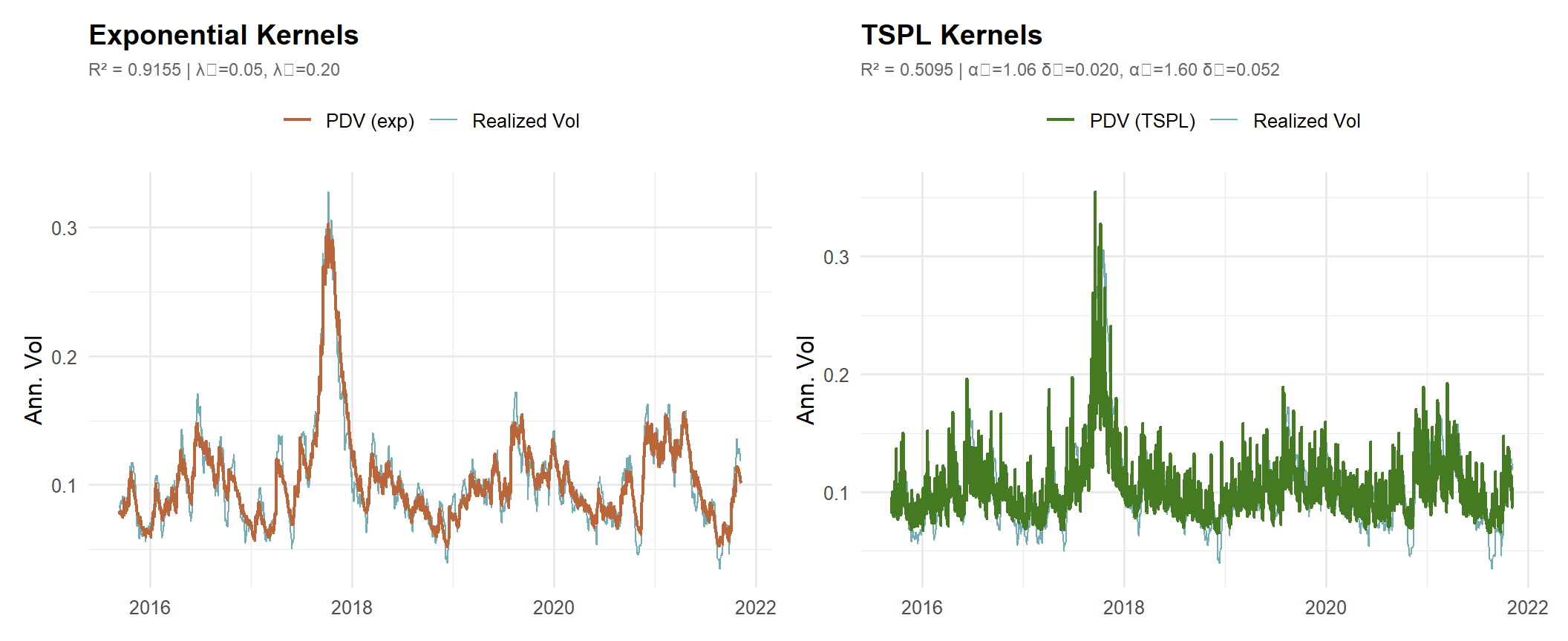

Roughness Check (Hurst Exponent)

Code

h_fitted <- compute_hurst(df_tspl$fitted)
h_true <- compute_hurst(true_vol)

tibble::tibble(
    Series = c("PDV fitted σ̂ (TSPL)", "True GARCH σ"),
    `H (simple R/S)` = c(h_fitted$Hs, h_true$Hs),
    `H (corrected R/S)` = c(h_fitted$Hrs, h_true$Hrs)
) |>
    mutate(across(where(is.numeric), \(x) round(x, 4))) |>
    knitr::kable(caption = "H < 0.5 = rough/anti-persistent. Paper reports H ~ 0.1.")

H < 0.5 = rough/anti-persistent. Paper reports H ~ 0.1.
Series	H (simple R/S)	H (corrected R/S)
PDV fitted σ̂ (TSPL)	0.7455	0.8864
True GARCH σ	0.7650	0.8811

Out-of-Sample Forecasting

Code

oos_forecast <- function(r, vol, train_end, kernel1_fn, kernel2_fn, K = 252, burn_in = 30, refit_every = Inf) {
    n <- length(r)
    w1 <- kernel1_fn(K)
    w2 <- kernel2_fn(K)

    wdot <- function(x, w) {
        m <- min(length(x), length(w))
        if (m == 0) {
            return(NA_real_)
        }
        sum(w[1:m] * rev(tail(x, m)))
    }

    make_df <- function(idx) {
        R1 <- vapply(idx, \(t) wdot(r[1:(t - 1)], w1), numeric(1))
        Sigma <- vapply(idx, \(t) sqrt(max(0, wdot(r[1:(t - 1)]^2, w2))), numeric(1))
        data.frame(t = idx, vol = vol[idx], R1 = R1, Sigma = Sigma)
    }

    train_idx <- seq(burn_in + 1L, train_end)
    train_df <- make_df(train_idx) |> na.omit()
    fit <- lm(vol ~ R1 + Sigma, data = train_df)

    test_idx <- seq(train_end + 1L, n)
    pred <- rep(NA_real_, n)

    for (i in seq_along(test_idx)) {
        t <- test_idx[i]

        if (is.finite(refit_every) && i > 1 && (i - 1) %% refit_every == 0) {
            refit_df <- make_df(seq(burn_in + 1L, t - 1L)) |> na.omit()
            if (nrow(refit_df) > 5) fit <- lm(vol ~ R1 + Sigma, data = refit_df)
        }

        R1_t <- wdot(r[1:(t - 1)], w1)
        Sigma_t <- sqrt(max(0, wdot(r[1:(t - 1)]^2, w2)))
        pred[t] <- predict(fit, newdata = data.frame(R1 = R1_t, Sigma = Sigma_t))
    }

    oos_df <- data.frame(
        t = test_idx,
        date = dates[test_idx],
        vol_actual = vol[test_idx],
        vol_pred = pred[test_idx]
    ) |>
        na.omit()

    oos_df$error <- oos_df$vol_actual - oos_df$vol_pred
    ss_res <- sum(oos_df$error^2)
    ss_tot <- sum((oos_df$vol_actual - mean(train_df$vol, na.rm = TRUE))^2)

    list(
        fit_is = fit,
        oos = oos_df,
        rmse = sqrt(mean(oos_df$error^2)),
        mae = mean(abs(oos_df$error)),
        r2_oos = 1 - ss_res / ss_tot,
        r2_is = summary(fit)$r.squared
    )
}

Run OOS (80/20 Split)

Code

train_end <- floor(0.8 * T_sim)

res_exp <- oos_forecast(
    r = r_sim,
    vol = realized_vol,
    train_end = train_end,
    kernel1_fn = function(K) exp_kernel(0.05, K),
    kernel2_fn = function(K) exp_kernel(0.20, K),
    K = K,
    burn_in = BURN,
    refit_every = Inf
)

res_exp_roll <- oos_forecast(
    r = r_sim,
    vol = realized_vol,
    train_end = train_end,
    kernel1_fn = function(K) exp_kernel(0.05, K),
    kernel2_fn = function(K) exp_kernel(0.20, K),
    K = K,
    burn_in = BURN,
    refit_every = 20
)

res_tspl <- oos_forecast(
    r = r_sim,
    vol = realized_vol,
    train_end = train_end,
    kernel1_fn = function(K) tspl_kernel(1.06, 0.020, K),
    kernel2_fn = function(K) tspl_kernel(1.60, 0.052, K),
    K = K,
    burn_in = BURN,
    refit_every = Inf
)

tibble::tibble(
    Model = c("Exp (static)", "Exp (rolling 20d)", "TSPL (static)"),
    `IS R²` = c(res_exp$r2_is, res_exp_roll$r2_is, res_tspl$r2_is),
    `OOS R²` = c(res_exp$r2_oos, res_exp_roll$r2_oos, res_tspl$r2_oos),
    `OOS RMSE` = c(res_exp$rmse, res_exp_roll$rmse, res_tspl$rmse),
    `OOS MAE` = c(res_exp$mae, res_exp_roll$mae, res_tspl$mae)
) |>
    mutate(across(where(is.numeric), \(x) round(x, 5))) |>
    knitr::kable(caption = "Out-of-sample performance summary")

Out-of-sample performance summary
Model	IS R²	OOS R²	OOS RMSE	OOS MAE
Exp (static)	0.81776	0.78896	0.01482	0.01200
Exp (rolling 20d)	0.81384	0.78756	0.01487	0.01203
TSPL (static)	0.60115	0.51502	0.02247	0.01827

OOS Forecast Plots

Code

make_oos_plot <- function(res, label, colour) {
    ggplot(res$oos, aes(x = date)) +
        geom_line(aes(y = vol_actual, colour = "Actual"), linewidth = 0.5, alpha = 0.8) +
        geom_line(aes(y = vol_pred, colour = label), linewidth = 0.8) +
        scale_colour_manual(values = c("Actual" = "#4f98a3", setNames(colour, label))) +
        labs(
            title = label,
            subtitle = sprintf("OOS R² = %.4f | RMSE = %.5f | MAE = %.5f", res$r2_oos, res$rmse, res$mae),
            x = NULL,
            y = "Ann. Vol",
            colour = NULL
        )
}

make_oos_plot(res_exp, "Exp (static)", "#bb653b") /
    make_oos_plot(res_exp_roll, "Exp (rolling)", "#7a39bb") /
    make_oos_plot(res_tspl, "TSPL (static)", "#437a22")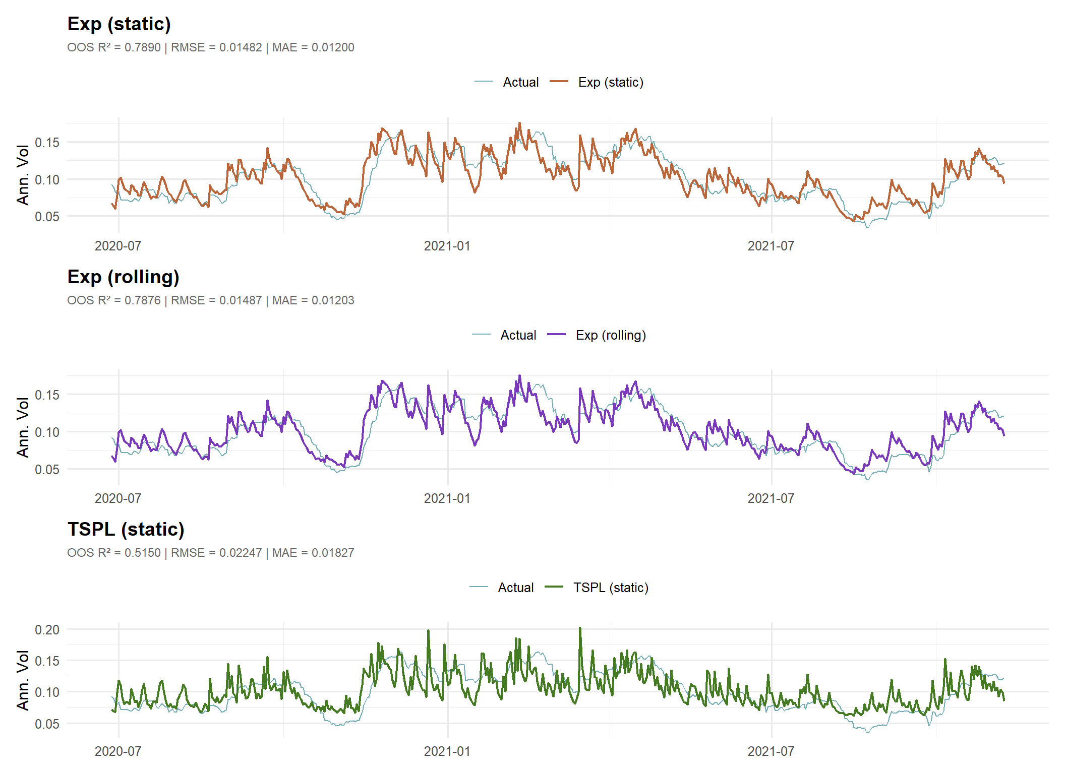

Error Distribution

Code

bind_rows(
    res_exp$oos |> mutate(model = "Exp (static)"),
    res_exp_roll$oos |> mutate(model = "Exp (rolling)"),
    res_tspl$oos |> mutate(model = "TSPL (static)")
) |>
    ggplot(aes(x = error, fill = model)) +
    geom_histogram(bins = 60, alpha = 0.7, position = "identity") +
    facet_wrap(~model, ncol = 3) +
    scale_fill_manual(values = c("#bb653b", "#7a39bb", "#437a22")) +
    labs(title = "OOS Forecast Error Distribution", x = "Actual − Predicted", y = "Count") +
    theme(legend.position = "none")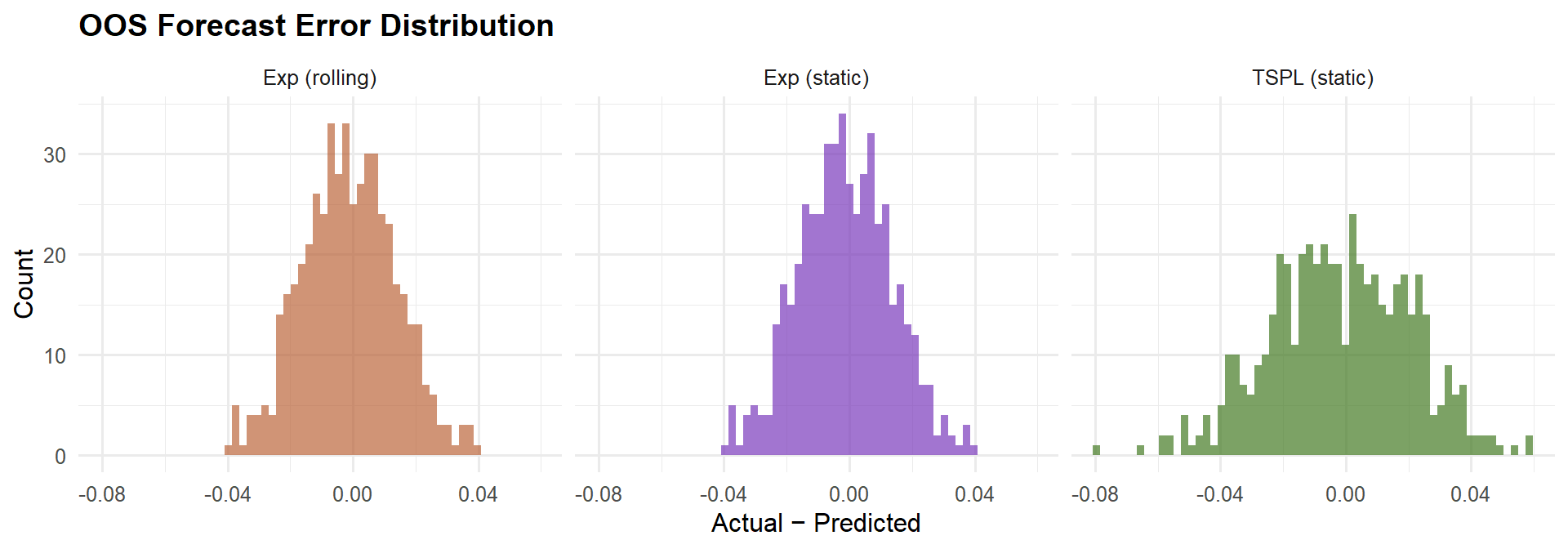

ACF of OOS Residuals

Code

acf_plot <- function(res, label, colour) {
    ac <- acf(res$oos$error, lag.max = 40, plot = FALSE)
    ci <- 1.96 / sqrt(nrow(res$oos))
    data.frame(lag = ac$lag[-1], acf = ac$acf[-1]) |>
        ggplot(aes(x = lag, y = acf)) +
        geom_col(fill = colour, width = 0.6) +
        geom_hline(yintercept = c(-ci, ci), linetype = "dashed", colour = "grey50") +
        labs(title = label, x = "Lag", y = "ACF")
}

acf_plot(res_exp, "Exp (static)", "#bb653b") +
    acf_plot(res_exp_roll, "Exp (rolling)", "#7a39bb") +
    acf_plot(res_tspl, "TSPL (static)", "#437a22")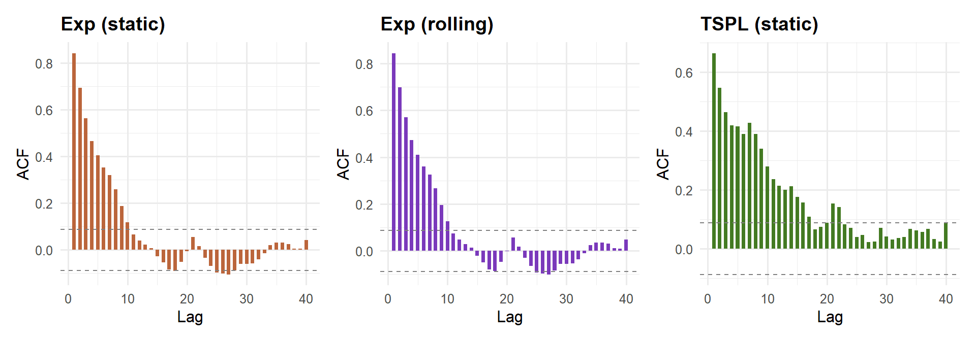

Plug In Real Data

Code

library(quantmod)

getSymbols("^GSPC", from = "2005-01-01")

[1] "GSPC"

Code

r_real <- as.numeric(dailyReturn(Cl(GSPC), type = "log"))
dates <- index(GSPC)

# Target 1: future realized vol
rv_target <- roll_vol(r_real, window = 21)

# Target 2: VIX (paper's primary target)
getSymbols("^VIX", from = "2005-01-01")

[1] "VIX"

Code

vix_target <- as.numeric(Cl(VIX)) / 100

n <- min(length(r_real), length(vix_target))
r_real <- r_real[1:n]
vix_target <- vix_target[1:n]

feats_real <- compute_features(
    r = r_real,
    kernel_fn = function(K) tspl_kernel(1.06, 0.020, K),
    K = 252
)
Sigma_real <- sqrt(pmax(
    as.numeric(stats::filter(r_real^2, tspl_kernel(1.60, 0.052, 252), sides = 1)),
    0
))

df_real <- data.frame(vol = vix_target, R1 = feats_real$R1, Sigma = Sigma_real) |>
    slice(-(1:30)) |>
    na.omit()

fit_real <- lm(vol ~ R1 + Sigma, data = df_real)
summary(fit_real) # expect R² ~ 0.90 for VIX target


Call:
lm(formula = vol ~ R1 + Sigma, data = df_real)

Residuals:
     Min       1Q   Median       3Q      Max
-0.34380 -0.05022 -0.01921  0.03393  0.62947

Coefficients:
            Estimate Std. Error t value         Pr(>|t|)
(Intercept) 0.147059   0.002079  70.740          < 2e-16 ***
R1          3.307203   0.472270   7.003 0.00000000000284 ***
Sigma       4.752134   0.169488  28.038          < 2e-16 ***
---
Signif. codes:  0 '***' 0.001 '**' 0.01 '*' 0.05 '.' 0.1 ' ' 1

Residual standard error: 0.08172 on 4951 degrees of freedom
Multiple R-squared:  0.1378,    Adjusted R-squared:  0.1375
F-statistic: 395.7 on 2 and 4951 DF,  p-value: < 2.2e-16